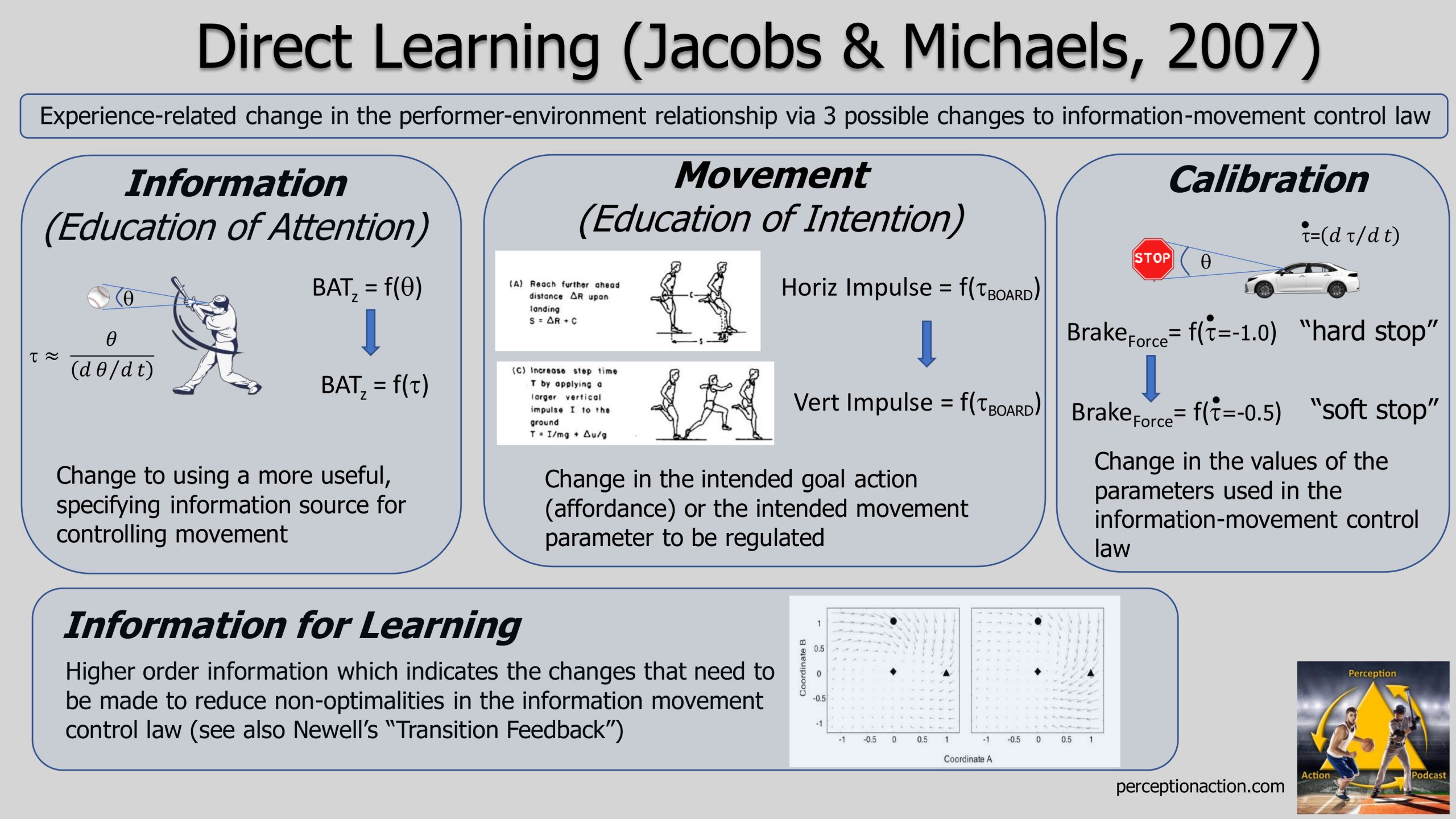
Overview: “Ecological theories hold that learning entails mere changes, for example, changes in which properties of ambient energy arrays perceptual systems respond to. Thus, in the ecological view, the sophistication of expert performance derives from the improved fits of experts to their environments, rather than from an increased complexity of computational and memorial processes. The learning theory that we explore in this article would indeed come under the heading of mere-change theories. The assumption that perception is a single-valued function of a single informational variable implies two types of change. First, change might occur in which informational variable is detected. In the present view, such change is said to be due to the education of intention or to the education of attention. Second, the particular single- valued function that carries the operative informational variable into perception might change. Such change may be due to calibration.” (Jacobs & Michaels, 2007)

Key Terminology & Definitions:

–Information-Movement Control Law– A coupling between a movement parameter (M) and an information source (I) of the form M=f(I), that if maintained will lead to success in producing the actor’s goal. The law describes how an action system functions at a particular moment.

–Education of Intention – A change in the intended goal action (i.e. the affordance to be realized) or the intended movement parameter to be regulated in the control law. An intention determines that the system acts the way it does, and therefore sets up the control law as a whole.

–Education of Attention – A change in the information used in control law to using (attending to) a more useful, specifying information source for controlling movement.

–Calibration – A change in the values of the parameters/constants used in the information-movement control law. Part of the calibration process involves changing to parameters that better take into account the action capabilities of the performer (e.g., maximum running speed).

–Information Space – Analogous to a state space for the coordination movement (explained here), an information space is a representation of possible combinations of information sources a performer could use in their movement solution.

Examples:

1) Timing a baseball swing
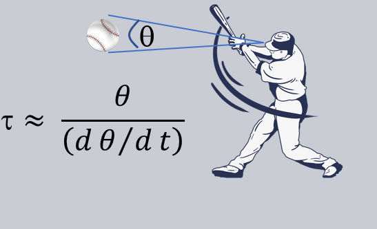
Imagine your goal is to try and hit a pitched baseball. To simplify things. let’s assume that your swing has a fixed movement time so that the movement parameter you intend to regulate in your control law is the initiation time (IT) of your swing. There a few different control laws, IT=f(I), you might use:

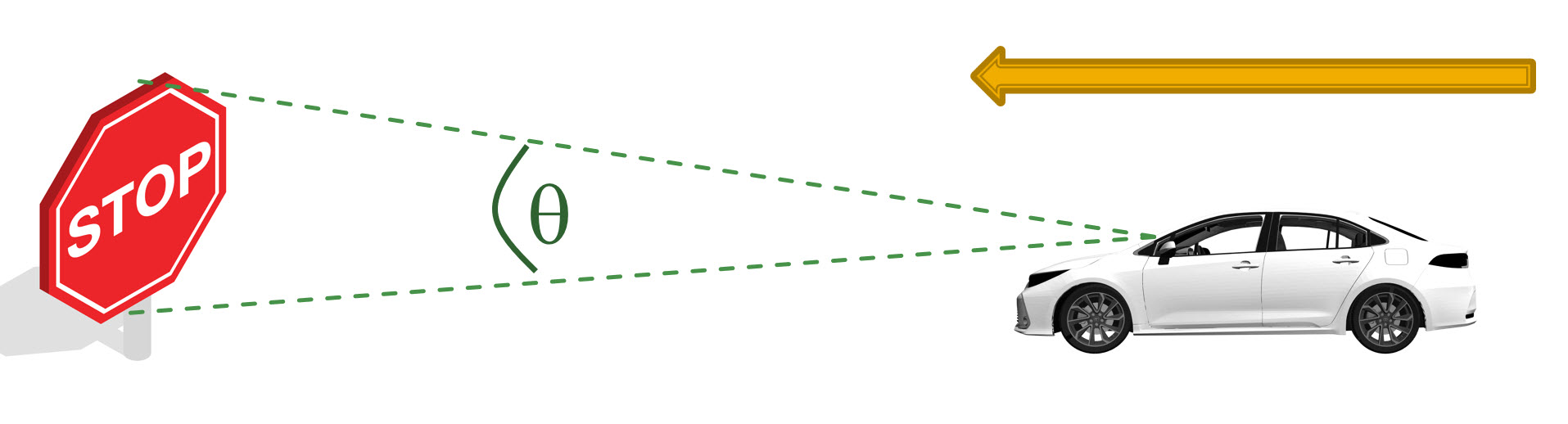
i)You could control your swing based on the distance of the ball (perceiving this from its angular size, θ) initiating your swing when the ball is a certain distance from you. So that the control law would be: IT = f(θ)

ii)You could control your swing based on the rate of expansion of the ball (dθ/dt) initiating your swing when it reaches a critical value: So that the control law would be: IT = f(dθ/dt)

iii)You could control your swing based on tau, which is a higher order variable created from the ratio of θ and dθ/dt. So that the control law would be: IT = f(Tau)

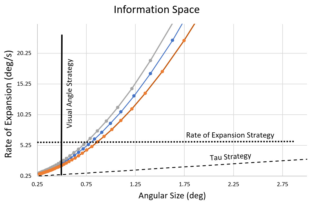
These different control laws along with the optical information created by the ball flight (the 3 colors show this for different pitch speeds) can be represented in an information space with θ and dθ/dt as the variables plotted on the axes:

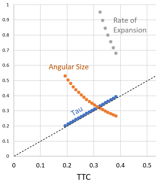
Importantly, in this situation, tau is a specifying variable because it directly specifies (i.e. directly relates to) the action relevant variable we need to achieve our goal – the time to contact (TTC) of the ball. On the other hand, θ and dθ/dt are non-specifying variables because the do not directly relate to TTC. This can be seen in the figure below:

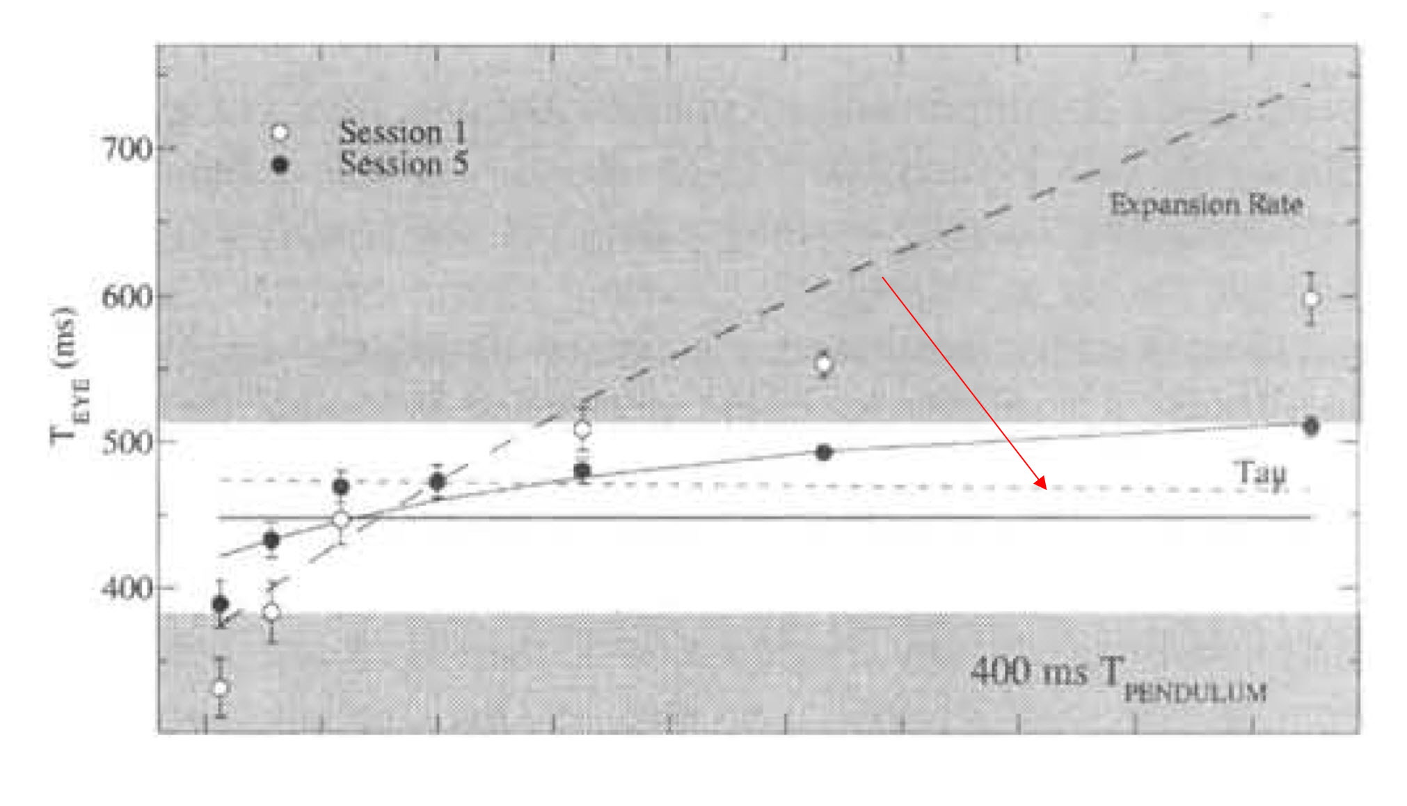
As found in an excellent series of experiments by Smith and colleagues, it is common for performers to use an interception strategy based on a non-specifying variable early in training then switch to a specifying one later with more practice at the task. This change is an example of education of attention to a new information source used in the control law. Here is an example from their study (note the information space is plotted with different variables). In session 1 (open circles) the interception data falls closer to the expansion rate strategy (thick dashed line) while after session 5 (closed symbols) it has shifted to fitting better with the tau strategy (fine dashed, horizontal line):

Critically, whether this education of attention occurs is strongly related to the variability of practice conditions. If the variability is too low there can be what Zhao and Warren call a visual-motor mapping in which a non-specifying information source can be effective for a narrow range of conditions. A classic example of this in baseball batting is hitting off a pitching machine set at a constant speed. In this situation the visual angle or rate of expansion strategies described above would be effective so the performer has no reason to educate their attention to use tau instead, which will be required in more realistic conditions where speed is varying.

2) Regulating the run up in long jumping

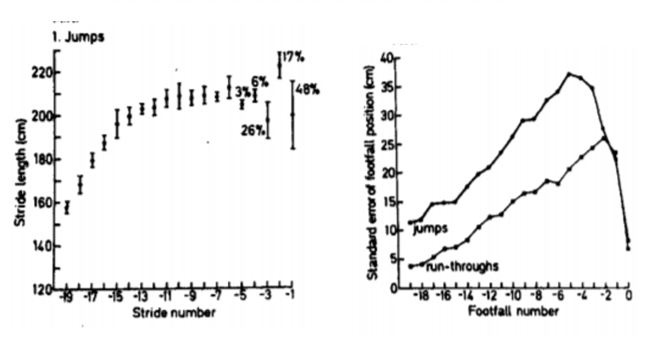
One of the keys in effective long jumping is to be able regulate your run up to the board so you hit it at a high speed without going over it. In the seminal study by Lee and colleagues, it was shown that long jumpers seem to do this by adjusting the length of their last few strides online using tau (in this case defined by the angle created between the long jumper’s eye and the board). This can be seen by the larger error bars on the left and the sudden drop in variability on the right in the figures below. In case you are interested I talked about this study in more detail in this video article review.

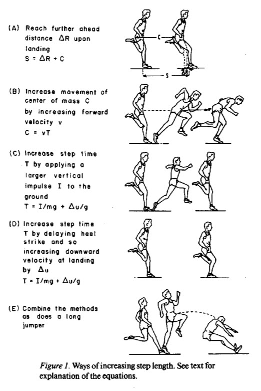
Therefore, in long jumping the control law is effectively: Stride Length (SL) = f(tau). But what parameter of the movement do we actually control to create different stride lengths? As described nicely in a paper by Warren, Young & Lee and illustrated in the figure below there are actually multiple ways you could do this (hello, Bernstein’s degrees freedom problem nice to see you again!). It can be achieved by varying the reach (or horizonal impulse) , how high you lift your legs (vertical impulse), leaning more or less, etc…

Studies looking at the effects of skill level on long jumping performance (e.g. Berg & Greer, 1995) have shown that one of things that seems to change with experience is which of these parameters is used to control stride length. For example, some athletes seem to switch from controlling it via horizontal impulse (HI) to altering vertical impulse (VI). So switching from HI=f(tau) to VI=f(tau). For me, this change is in an example of education of intention because the performer is changing the movement parameter they intend to control without changing the information used.

3) Braking a car
When braking a car at a stop sign we need to control rate of deceleration based on the visual information. As first shown by David Lee, one way this can be achieved is by coupling the brake force we apply to the variable tau-dot, which is the rate of change of tau (θ/(dθ/dt)). Therefore, we could write the basic control law as: Force (F) = f(tau-dot).

But, as anyone who has rented a car will have experienced, brake pedals are not all built the same. Specifically, the relationship between the force you apply on the brake and the rate at which the car decelerates is different for different cars. Some are very sensitive others have “spongy” pedals that you have to push much harder. We can take this into account in our control law by adding a calibration parameter, a. So, our new control law becomes F=a*tau-dot.

Brett Fajen has shown in an excellent series of studies, that drivers can quickly adjust this calibration parameter to learn to drive a car with different brake dynamics. For example, in a 2007 study, 3 groups initially (for the first 5 blocks) drove cars with very different braking abilities. As shown below, they all stopped successfully by using different calibrations between information and movement. On trial 6, they were all switched to a car with same braking dynamics. As you can see, they rapidly (within 2 blocks) recalibrated their control law.

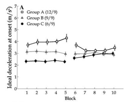
This is an example of the final way we can learn from experience, calibration. We can change how the movement parameters and information sources are coupled without changing the movement we are controlling or the information we are using.

Information for Learning:

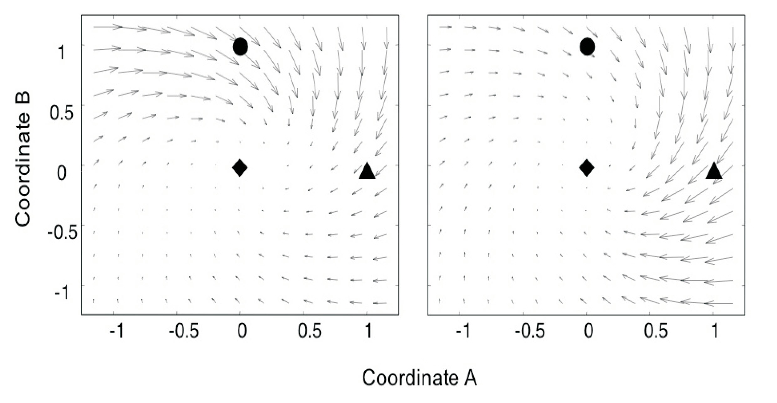
This most bold claim made in Jacobs & Michaels direct learning theory is that not only is there specifying information directly available from our environment that we can use to control our actions (Gibson’s fundamental idea) but there is also direct information that guides learning. Stated another way, there is information available that tells us what changes we need to make in our control laws to make them better. Conceptually, this seems to be very similar to Newell’s concept of transition feedback, which I discussed here. The authors represent this as vector fields in the information spaces that point you in the direction you need to go.

This is an idea I will be discussing more in the future. But you can also check out Andrew Wilson’s excellent initial evaluation of the ideas here.

Articles – Theoretical Foundations:
–Direct Learning
–The direct learning theory: a naturalistic approach to learning for the post-cognitivist era

Articles – Empirical Research:
–Learning to visually perceive the relative mass of colliding balls in globally and locally constrained task ecologies
–The Learning of Visually Guided Action: An Information-Space Analysis of Pole Balancing
–Monocular optical constraints on collision control
–The Education of Attention as Explanation of Variability of Practice Effects: Learning the Final Approach Phase in a Flight Simulator
–Lateral interception I: Operative optical variables, attunement, and calibration
–Lateral interception II: predicting hand movements
–Learning to Avoid Collisions: A Functional State Space Approach
–Self-controlled concurrent feedback and the education of attention towards perceptual invariants

Blogs:
–Direct Learning (Jacbos & Michaels, 2007)
–Evaluating ‘Direct Learning’

Podcast Episodes:
–53 – Perceptual Learning II – Direct Learning

Video Presentations: